Most (if not all) programming languages have random number functions that produce uniformly distributed values. What about random numbers from an arbiutrary, non-unform distribution?

In this post we’ll explore several methods to generate random numbers from a Normal distribution. To simplify things a bit we’ll work with a standard Normal distribution. This distrubtion has a mean $\mu = 0$, and a standard deviation $\sigma = 1$. This choice doesn’t limit us in any way because there’s a one-to-one mapping between the standard Normal distrubtion and any other normal distribution with the mean of $\mu$ and variance of $\sigma$:

Method 1: Central Limit Theorem

Central limit theorem states that the mean of a sum of samples from any distribution approaches normal distribution as the size of the sample increases. This is really cool. Regardless of how our original values are distributed, if we sum them up we get an (approximate) normal distribution!

As little as ten elements in a sample is sufficient to approximate the normal distrubution quite closely. Here’s the plan:

1. Generate 10 samples from our uniform random numbers generator.
2. Sum them up.
3. Repeat this process 10,000 times to obtain 10,000 normally distributed samples.
4. Plot our distribution and compare it to the theoretical normal distribution to see if we got the right result.

Below is the annotated code in R language. You can easily re-implement this in any other language.

The number of samples per iteration is 10:

sample_n = 10 # We will draw samples form the uniform distribution

The number of values from a Normal distibution:

n = 10000 # The number of normal samples

Generate 10 x 10,000 total random numbers from a uniform distribution $[0, 1]$:

uniform_samples = runif(n = sample_n * n, min = 0, max = 1)

Reshape uniform_samples array into a matrix with 10,000 rows and 10 elements in each row:

samples_matrix <- matrix(uniform_samples, nrow=n, byrow = T)
head(samples_matrix, n = 2)

##           [,1]      [,2]      [,3]      [,4]      [,5]      [,6]      [,7]
## [1,] 0.2092528 0.5840815 0.7347990 0.5423473 0.1061720 0.3642399 0.2826386
## [2,] 0.5755127 0.7354924 0.4201131 0.6875674 0.1339724 0.4634930 0.1218253
##           [,8]        [,9]     [,10]
## [1,] 0.8271714 0.043840417 0.8085010
## [2,] 0.5757191 0.002331376 0.4328097

Now we calculate the mean of each row to get a normally distributed varible, per Central Limit Theorem. We use the mean instead of the sum for convenience. In our case the mean is simply the sum divided by 10 (the number of values in each row), so either value will stil be a normally distributed variable.

x <- rowMeans(samples_matrix)

According to the Central Limit Theorem our constructed normal distribution will approximate the normal distibution with mean $\mu = \mu_{sample}$, or $\mu = 0.5$, and with standard deviation $\sigma = \sigma_{sample} / \sqrt{n}$, where $n$ is the number of values in each sample, i.e. 10.

mu = 0.5
sigma = sd(uniform_samples) / sqrt(sample_n)
normal_x = (x - mu) / sigma

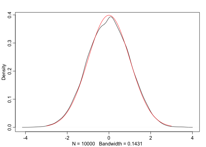
dens(normal_x, adj = 1)
true_normal.x <- seq(-3, 3, length.out = 100)
true_normal.y <- dnorm(true_normal.x, mean=0, sd=1)
lines(true_normal.x, true_normal.y, col="red")

Inverse Transform Sampling

Inverse transform sampling relies on the fact that if $X$ is a random variable from any disribution, $F$ is its cumulative distribution function (i.e. $F(x)$ is the probability of the value being $\le x$ ) then $F(x)$ is distributed uniformly. Let’s test this statement:

inverse_transform <- function () {
  samples <- rnorm(n = 100000, mean=0, sd=1)
  cdf <- pnorm(samples)
  dens(cdf)
}
inverse_transform()

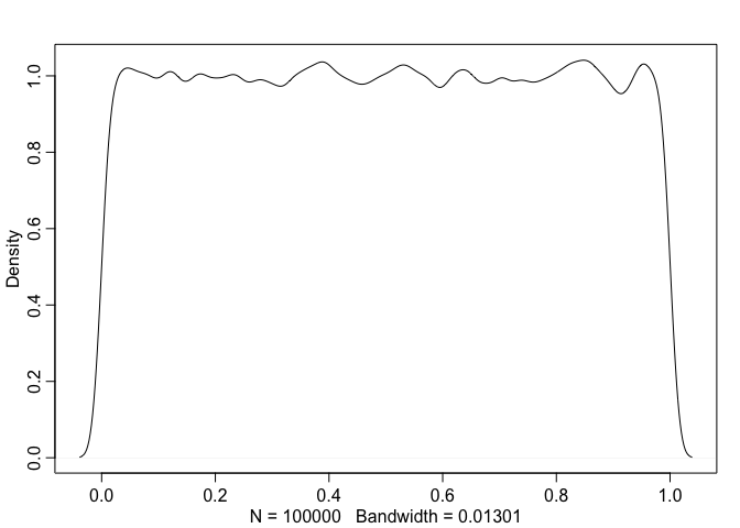
Indeed, a cumulative distribution function of our normally distributed variable is approximately uniform. So, if we know a CDF $F$ for a Normal distribution, we can generate samples from the Normal distribution via the following steps:

1. Generate samples $u$ from the uniform distribution
2. Calculate $x = F^{-1}(u)$, where $F$ is the CDF for the Normal distribution. Then $x$ will be normally distriubted.

However, this method is not very efficient for continuous cases where the cumilative distribution function $CDF$ doesn’t have an analytic integral. Normal distribution is such an example. Because of this, other methods are more popular.

Box-Muller Transform

The Box-Muller Transform algorithm transforms two uniformly distributed variables into two normally distributed variables. The implementation is below.

First, let’s define some constants:

eps = .Machine$double.eps
two_pi = 2 * 3.141592653589793

The number of normally distributed samples we want to get:

n = 10000

Generate uniform samples, 5,000 rows x 2 samples in each row, the total of 10,000 samples:

uniform_samples = runif(n = n, min = 0, max = 1)
samples_matrix <- matrix(uniform_samples, nrow=n / 2, byrow = T)
head(samples_matrix, n = 2)

##           [,1]      [,2]
## [1,] 0.7127697 0.3939681
## [2,] 0.6738139 0.7353309

Apply the Box-Muller transform to obtain normally distributed samples. Both variables $z_{0}$ and $z_{1}$ will be normally distributed:

z0 = sqrt(-2 * log(samples_matrix[,1])) * cos(two_pi * samples_matrix[,2])
z1 = sqrt(-2 * log(samples_matrix[,1])) * sin(two_pi * samples_matrix[,2])
head(z0)

## [1] -0.646948983 -0.081784960  0.946564142 -0.003156047  0.591291990
## [6]  1.919719021

Let’s combine $z_{0}$ and $z_{1}$ into a single array $z$, plot the density function of $z$, and compare it to the true normal distribution:

z = cbind(z0, z1)
dens(z, adj = 1)

true_normal.x <- seq(-3, 3, length.out = 100)
true_normal.y <- dnorm(true_normal.x, mean=0, sd=1)
lines(true_normal.x, true_normal.y, col="red")

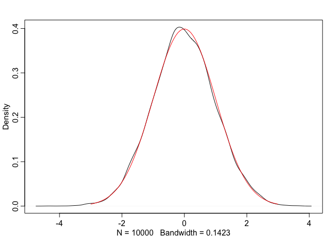
As we can see, Box-Muller transform indeed produces normally distributed values.